Introduction
Hello reader this is a short summary of our notes about the course “Biochip”. If you find an error or you think that one point isn’t clear please tell me and I fix it (sorry for my bad english). -NP
Chapter Zero: Bases
Definition of Biosensor: A (chemical) sensor based on a biological entity.
Biosensor work with an Analyte and Receptors:
- Analyte: target molecule;
- Receptors: Receive the target and bind with it.
Analyte \xrightarrow{bind} Receptor \xrightarrow{change} Electronic transformation
Planar configuration: Receptor is immobilized on the sensor.
Technological issue: how to attach the molecule to a solid substrate while presenting its function (in a liquid environment) \implies chemical functionalization.
Geometrical Parameters (for simplify analysis):
- Contour Length (L): length of the macro molecule backbone.
- Radius of gyration (R_g): for a folder, globular macromolecule is the average between the extremes.
Motion of fluids \to Navier-Stokes
We work with fluids + particles and simple fluids.
Chapter One: Fluids Law
Main properties of fluid:
- Density (\rho)
- Viscosity (\eta)
- Surface tension (\gamma)
Simple fluids:
- Newtonian
- Non-Newtonian
Complex fluids:
- Electrolytes: simple fluids + ions in solution
- Suspensions: simple fluids + large particles
- Complex fluids: fluids + heterogeneity change the properties
1.1 Properties
Density: \rho = \frac{\text{Mass}}{\text{Volume}}[\frac{kg}{m^3}] \implies important to set flowing and sedimentation time of particles \to decrease with temperature (higher is the temperature lowest is the density)
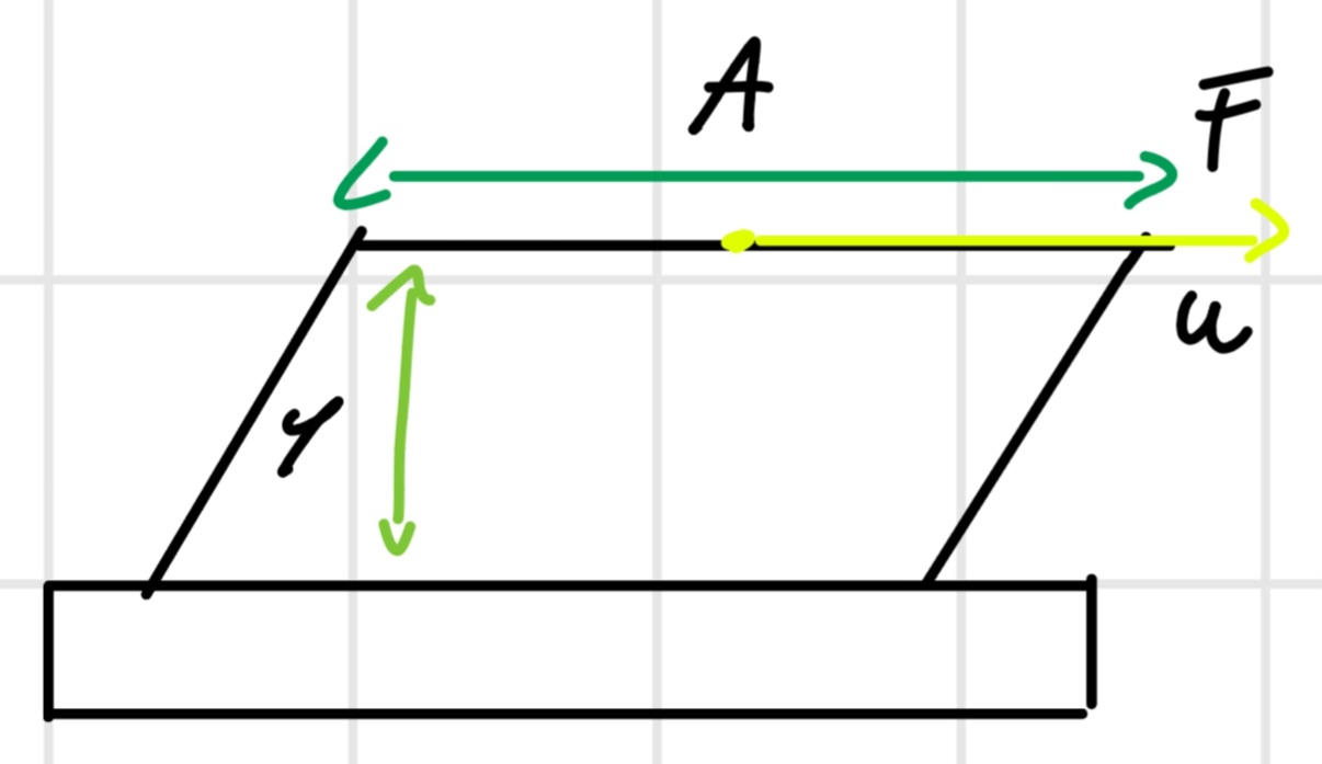
Viscosity: \eta = \frac{F}{A} * \frac{y}{u} [P_a * s] but \frac{F}{A} is called shear stress \tau \to \eta = \tau * \frac{y}{u} \implies Express the resistance to deformation by \tau
- F: force applied to win the resistance and to maintain a constant velocity u of top plate (Area A)
- u: velocity
Viscosity increase with the temperature (low temperature, high viscosity)
\eta (T) = \eta_0 e^{-bT}
Viscosity of blood estimates greater than water (5,5 vs 1)
Non-Newtonian fluids
- Newtonian like water: \eta independent by \tau
- Non-Newtonian like blood: \eta dependent by \tau
Pseudo-Plastic: non-newtonian at some point the \eta decrease and it’s simplest to move (honey)
Dilatant: non-newtonian at some point the \eta increase and it’s hardest to move
1.2 Flow Regimes
Laminar Flow
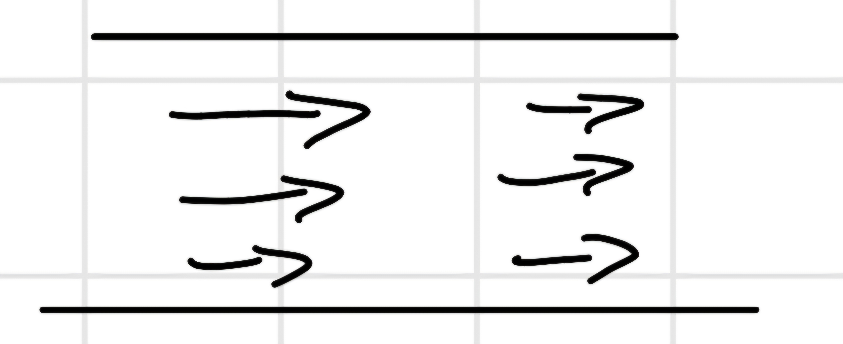
- No turbulence
- Reversible
- Minimum dissipation
- Unique solution
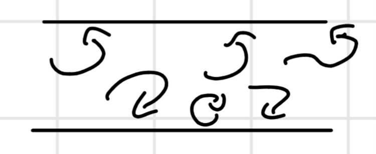
Turbulent Flow
Chaotic flow with vortex
Reynolds Number: R_e = \frac{\rho * 2r * v}{\eta}
- v: fluid velocity [\frac{m}{s}]
- r: channel radius [m]
- \rho : density [\frac{kg}{m^3}]
- \eta : viscosity [P_a * s]
R_e < 2300 laminar flow.
R_e > 3000 turbulent flow.
We work with R_e < 1 usually
For non-circular conduits we use an approximation to work to an equivalent circular radius
r_{eq} = \frac{2*Area}{Perimeter}
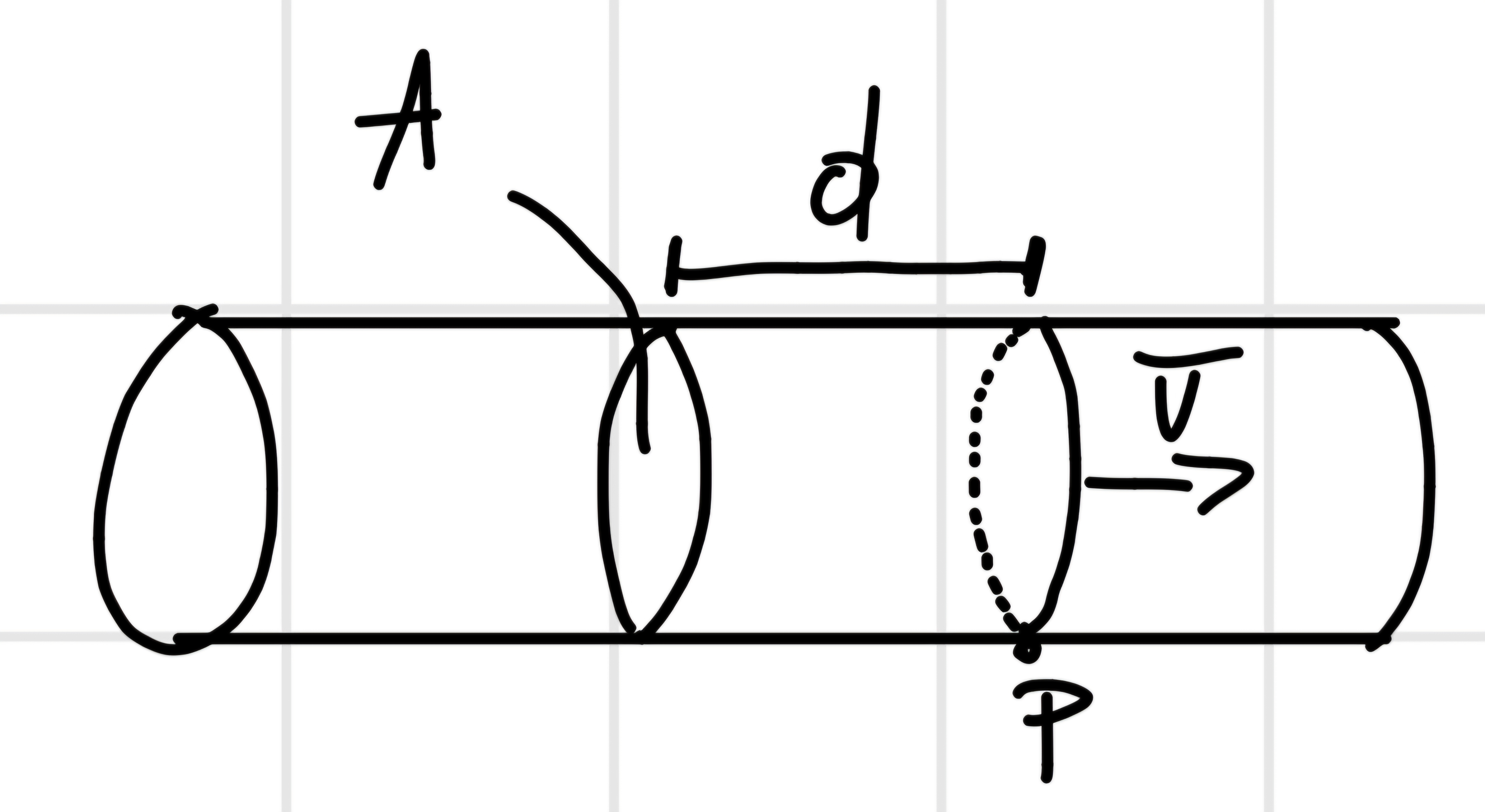
\overline{v} = \frac{d}{t}
Q = \frac{V}{t} = \frac{A*d}{t} = A*\overline{v}
- Q: Volumetric flow rate [\frac{m^3}{s}]
- V: Volume = A*d
- v: velocity
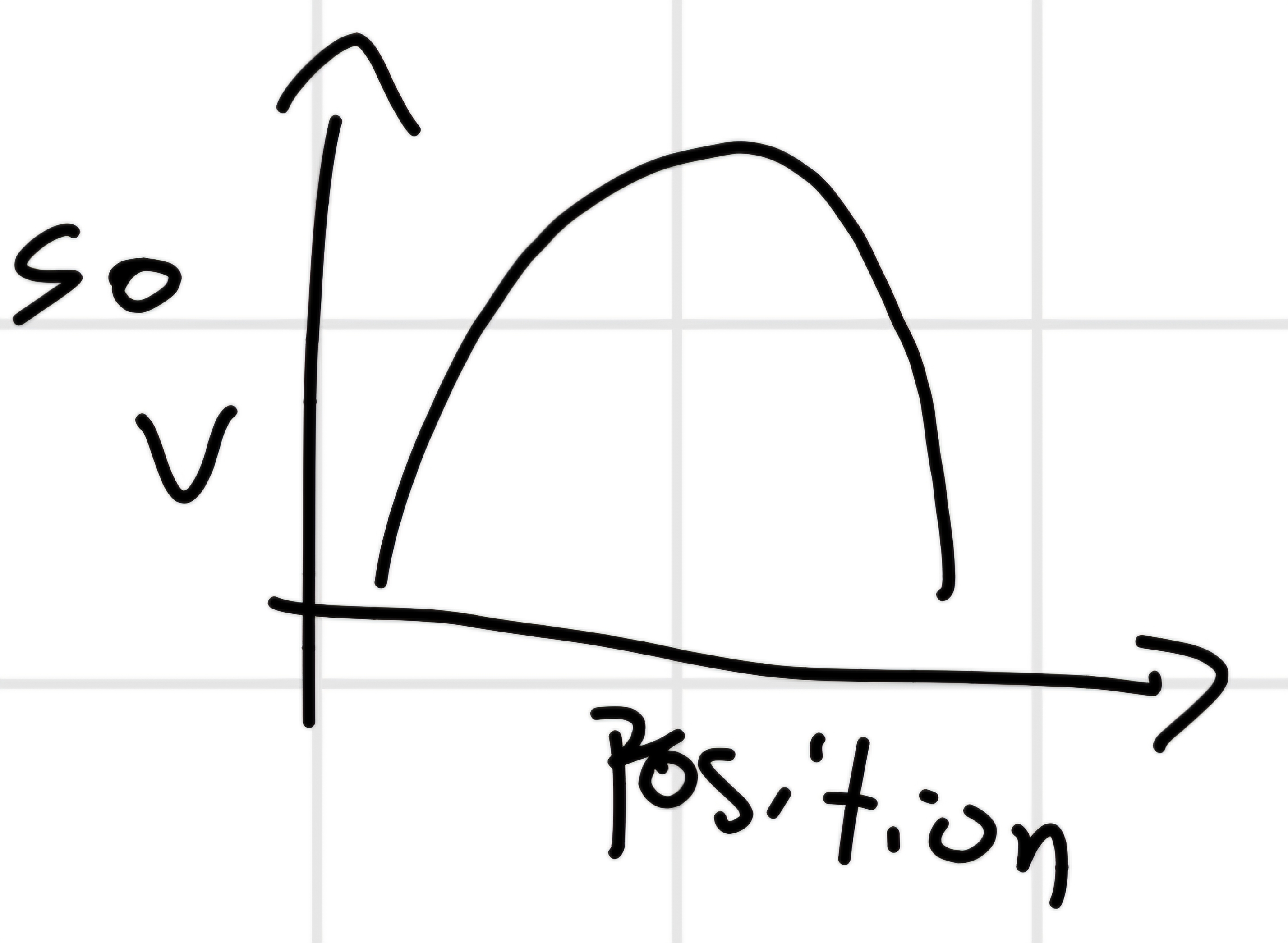
1.3 Velocity profiles
For pressure-driven laminar flow, the no slip condition at the conduit walls implies that v=0 \implies parabolic velocity profiles.
We have difference due the slip with the wall, so:
The velocity change with the channel changes
1.4 Resistance to Flow
The energy dissipated in the friction of the fluid against the conduit walls requires a pressure difference \Delta P to create a flow rate Q [\frac{m^3}{s}]
Poiseuille law: Q = \frac{\Delta P}{R}
R: fluidic resistance, depends on the conduit section [\frac{P_a * s}{m^3}]
The analogous of Q is I = \frac{\Delta V}{R}, will be a lot of analogy with electronic law and fluids one.
How calculate R know the characteristic of the conductor:
R = \frac{8*\eta*L}{\pi * r^4} [\frac{P_a * s}{m^3}]
Whit rectangular section (so, without approximation)
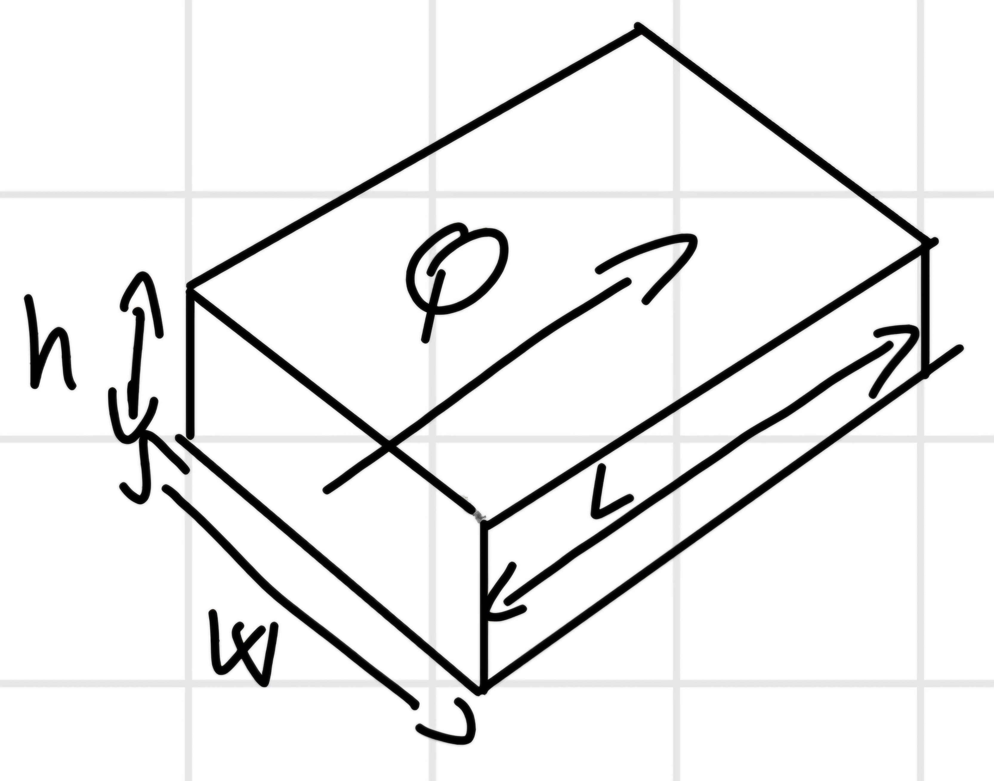
R = \frac{12* \eta * L}{C(\frac{w}{h}) * h^3 *w}
C: friction factor.
So in our case, if \frac{w}{h}>1,4 use the formula without approximation, otherwise the other one.
C(\frac{w}{h}) = (1 - 0,63 \frac{h}{w})
Mass conservation Law: like Kirchhoff
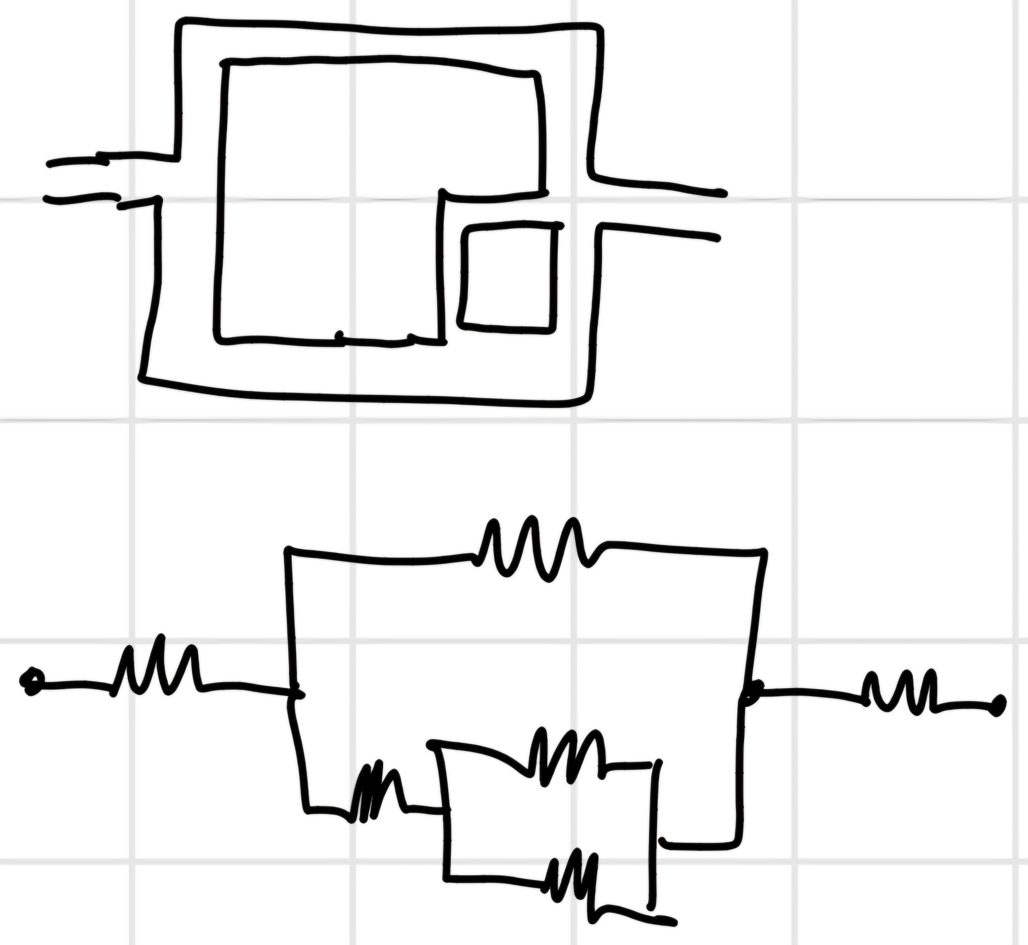
We can use the same law of the conservation of voltage in the fluids case.
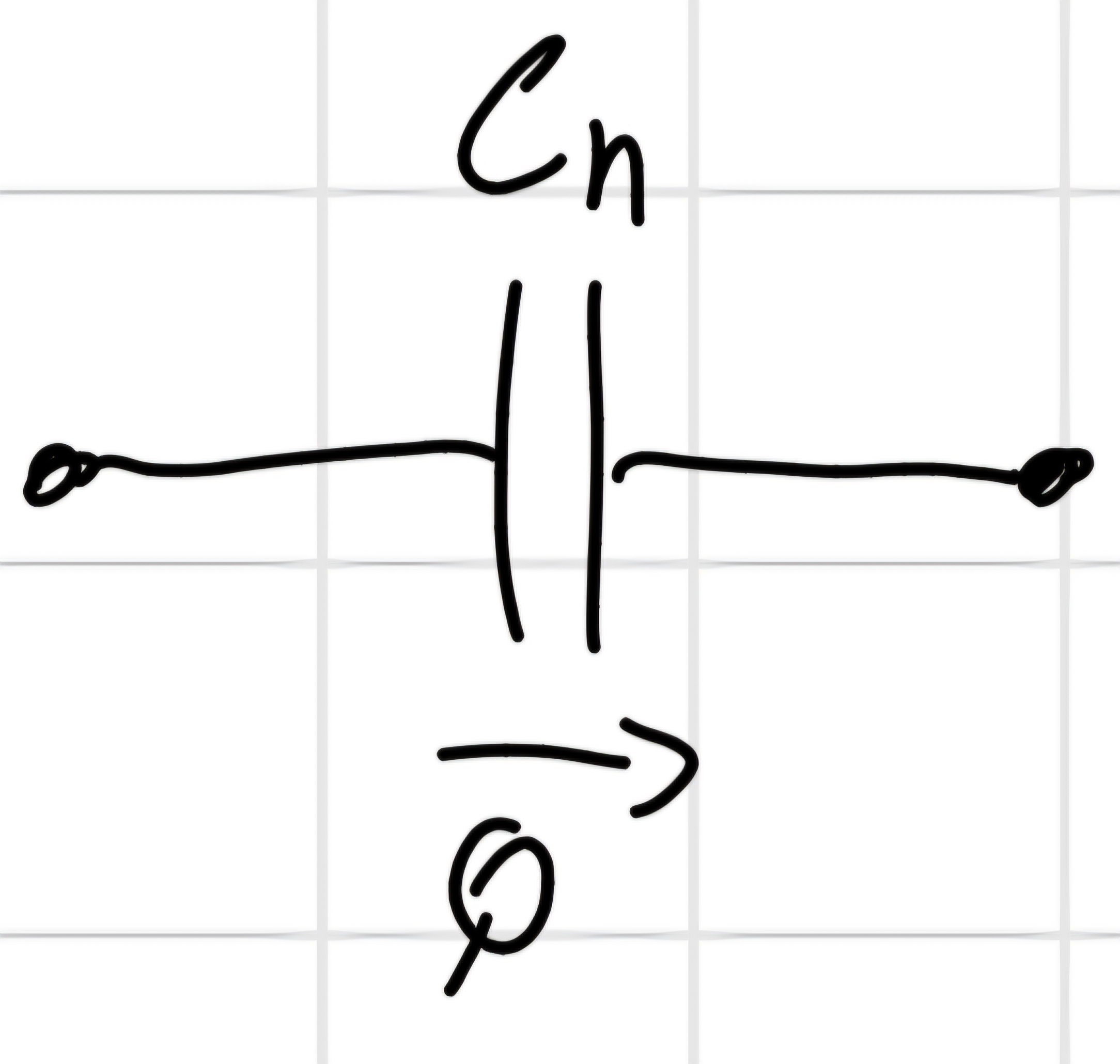
1.5 Hydrodynamic Capacitance
Q = C_h \frac{d \Delta P}{dt}
C_h = \frac{\int{Q(t) dt}}{\Delta P} = \frac{Volume}{\Delta P} [\frac{m^3}{P_a}] \implies analogous with electronic capacity.
Time constant: R_h * C_h [s]
Type of walls:
- Rigid wall, incompressible C_h = 0
- Rigid wall, incompressible fluid, bubble with ideal gas: C_h = \frac{p_0 * V_0}{p^2}
- Flexible wall, incompressible fluid: C_h is a function of geometry and material properties.
1.6 Surface Tension
Force necessary to break the surface
F = 2\gamma * L + mg
\gamma: surface tension coefficient [\frac{N}{m}]
Meniscus in a capillarity
- Concave F_{\text{adhesion}} > F_{\text{cohesion}}
- Convex F_{\text{adhesion}} < F_{\text{cohesion}}
POV of the surface
Wettability: Ability of a liquid to adhere to a solid surface.
In case of water, the surface can be:
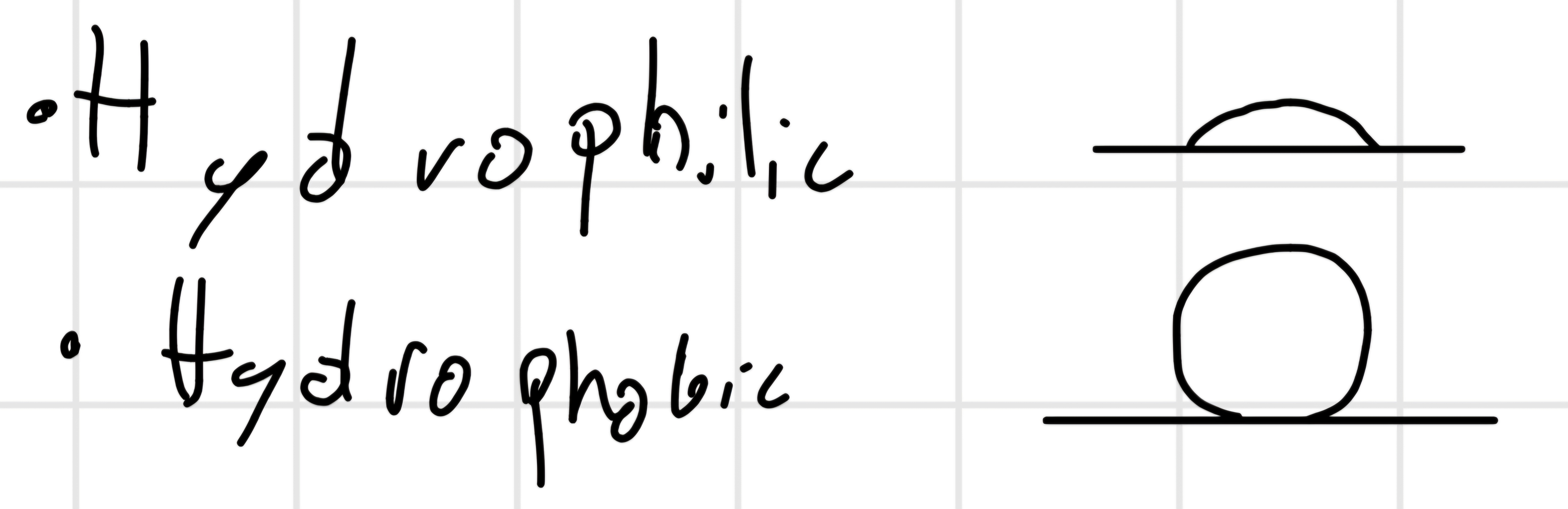
We can determine the wettability using the contact angle \theta_c
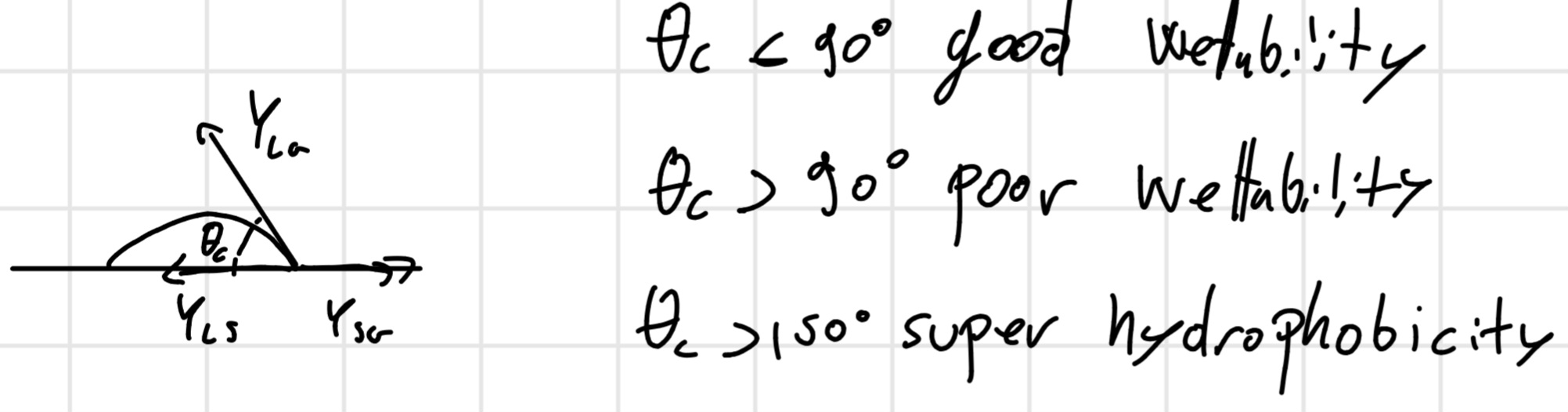
It possible uses the electricity to modify the surface wettability, liquid must contain ions.
1.7 Forces in Micro fluidic system
1.7.1 Diffusion
If we put a drop of ink in a cup of water, we can see the diffusion \implies Brownian motion \to tends to the equilibrium with a random walk.
A spatial gradient of molecule (mass) concentration C[\frac{kg}{m^3}]
Fick’s law: J = -D \frac{\partial C}{\partial x}
D: diffusion coefficient [\frac{m^2}{s}]
J: \frac{\partial m}{\partial t \partial A}
L_{diff} = \cong \sqrt{D t}
Diffusion coefficient: D = \frac{k*T}{6*\pi*\eta*r} \to spherical particles at low R_e
Diffusion time is a lot, diffusion is slow:
- L = 1cm \to \Delta t = 7 hours.
- L = 10 \mu m \to \Delta t = 25 ms at minus scale is acceptable.
1fM \implies D = 1,5*10^{-6} \frac{cm^2}{s}
Peclet Number: P_e = \frac{v * L}{D}
- v: fluid velocity;
- L: length scale;
- D: diffusion coefficient.
Quantitative figure of merit of the competition between forced flow and diffusion transport.
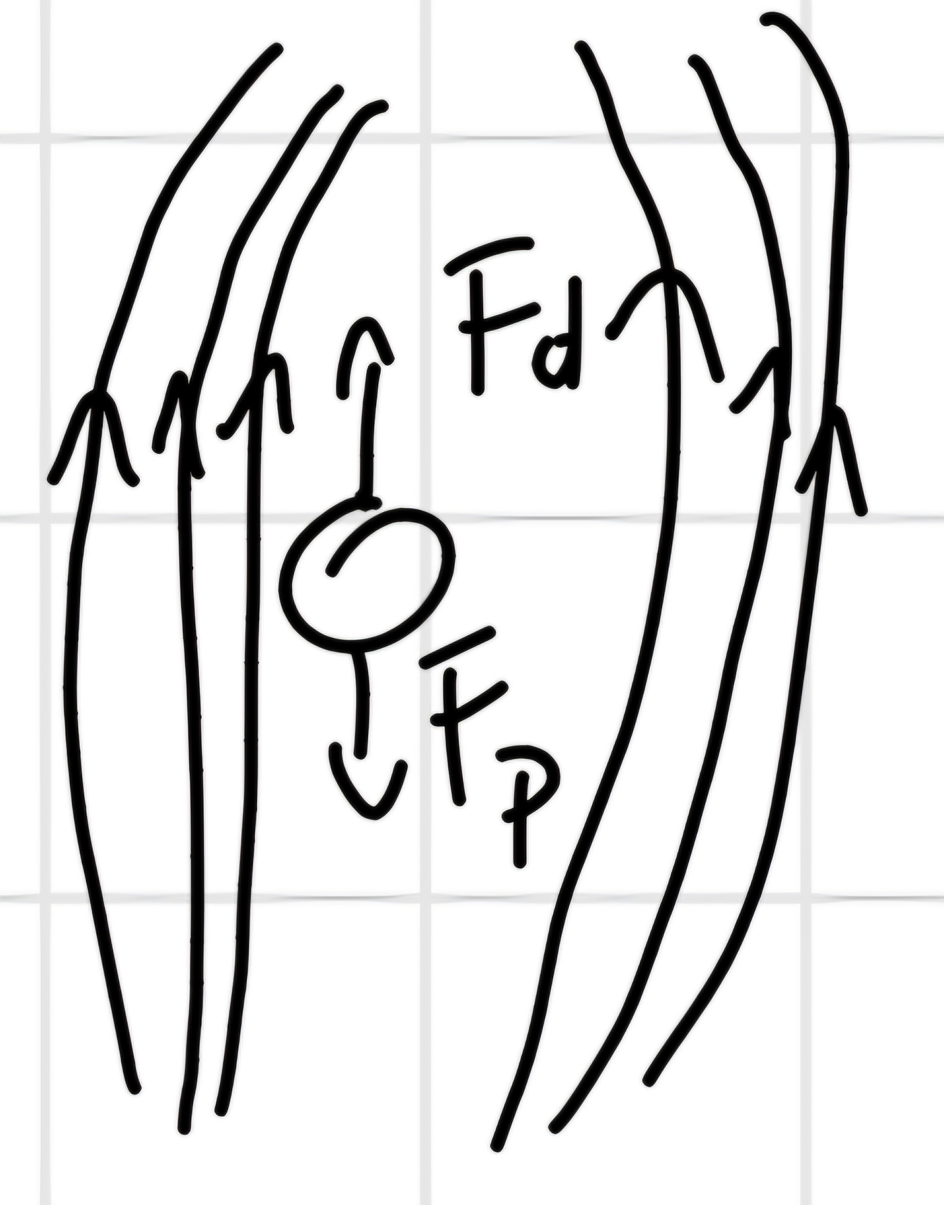
1.7.2 Drag Force
A particle moving in a viscous fluid (viscosity \eta) with relative velocity v \to friction force (drag).
For spherical particles of radius r and R_e low: F_{drag} = -6 * \pi * \eta * r * v
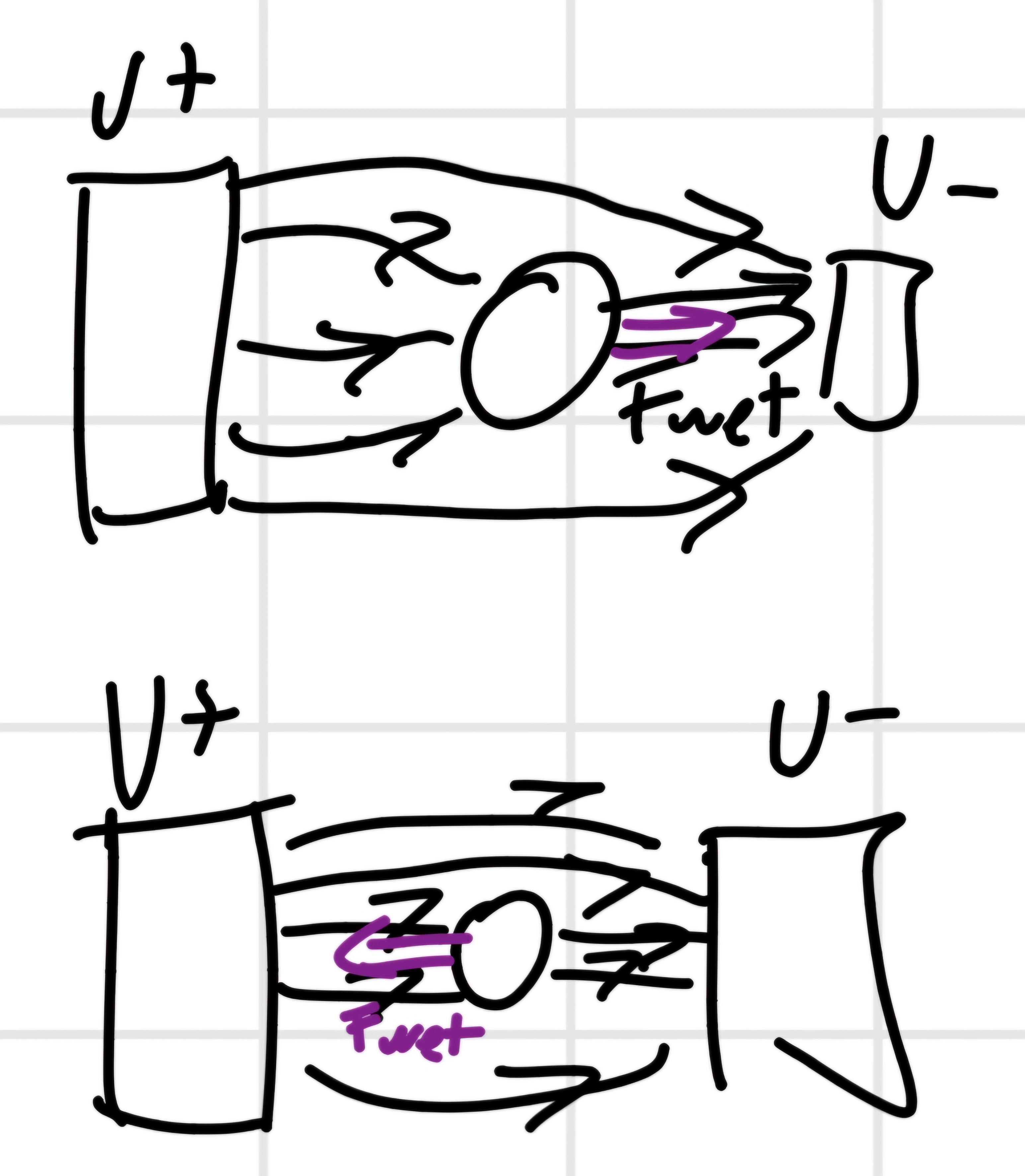
Electrokinetics: Electrostatic Coulomb force on a charged particle (q) immersed in an electric field E
F_E = q* E = F_d = 6 \pi \eta r v \implies migration velocity: v = \frac{q}{6 \pi \eta r} E = \mu * E \to \mu = \frac{q}{6 \pi \eta r}
\mu: electrophoretic mobility
In constant E, the transit time depends on the mobility of the molecule. \mu \cong \frac{q}{r}, depends on the size.
In this case we don’t use water but gel \to higher viscosity.
1.7.3 Dielectrophoresis (DEP)
Neutral dielectric particles in liquids can moved by means of DEP, a net force that acts on the particle in a non-uniform electric field (gradient).
- Polarization: ability of the particle to be polarized in an external field E, \vec{p} = \alpha \vec{E}
\alpha = \frac{\vec{p}}{\vec{E}} [\frac{cm^2}{V}]
- Permittivity: every material have a permittivity constant, \varepsilon, to study the function of frequency we need the complex one, \varepsilon^* = \varepsilon + \frac{\sigma}{jw}
\sigma: conductivity
- DEP Force: \vec{F} = \vec{P} * \nabla E = \alpha * \nabla E^2
For homogeneous spherical particle (radius r, permittivity \varepsilon_p) in a surrounding medium \varepsilon_m the force is:
\vec{F} = 2 *\pi * r^3 * \varepsilon_m * Re\{K_{CM}(w)\} * \nabla E^2
Clausius-Mossoni Factor: K_{CM}(w) = \frac{\varepsilon_p^* - \varepsilon_m^*}{\varepsilon_p^* + 2*\varepsilon_m^*}
Re\{K_{CM}(w)\} \to DEP force.
Im\{K_{CM}(w)\} \to Electrorotation.
Digital Microfluidics \to based on the manipulation of single droplets.
2 way:
- Channel based;
- Surface based.
How manipulate one droplets:
- Fluids (pomps and same way seen);
- Electrowetting, use electricity to move the droplet cos(\theta) = cos(\theta_0) + \frac{1}{2*\gamma} C * V^2